The EWorldShape object In a general content, the term object should be understood with the meaning of a class instance. In EasyObject, an object is a maximally-sized area of adjacent connected pixels belonging to the layer foreground. can calibrate the whole field of view (in given imaging conditions with fixed camera placement and lens magnification), if the optical setup is modified.
EWorldShape computes appropriate calibration coefficients and transforms measurement gauges that are tied to it.
It can set world-to-sensor transform parameters, perform conversions from and to either coordinate system, determine unknown calibration parameters, and save the parameters of a given transform for later reuse.
After calibration EWorldShape can perform coordinate transform for arbitrary points using SensorToWorld and WorldToSensor to:
| □ | measure non-square pixels and rotated coordinate axis. |
| □ | correct perspective and optical distortion, with no performance loss. |
There are several ways to obtain the calibration coefficients:
Estimate (feasible if no distortion correction is required and accuracy requirements are low)
To estimate the calibration coefficients either locate the limits of the field of view and divide the image resolution by the field of view size, or use the following procedure:
| 1. | Take a picture of the part to be inspected or a calibration target (e.g. rectangle). |
| 2. | Locate feature Geometrical property of a coded element. points such as corners in the image (by the eye) and determine their coordinates in pixel units —let (i,j). |
| 3. | Use the euclidean distance formula to derive the calibration coefficient: 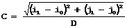 where C is a calibration coefficient, in pixels per unit, and D is the world distance between the corresponding points, in units. |
| 4. | For non-square pixels repeat this operation for pairs of horizontal and vertical points. |
To estimate a skew angle, apply this formula to two points on the X-axis in the world system: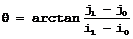

Estimating scale factors and skew angle
When the calibration coefficients are available, use SetSensor to adjust them and set the calibration mode, or set them individually using: SetSensorSize, SetFieldSize, SetResolution, SetCenter, SetAngle.
Pass a set of reference points (landmarks) to a calibration function
Locate at least 4 landmarks and obtain their coordinates in sensor (using image processing) and world coordinate systems (actual measurements). More landmarks give more accurate calibration.
The resulting pixels aspect ratio (X resolution / Y resolution) must be in the range [-4/3, -3/4] (or [3/4, 4/3]).
Use the method EWorldShape.AddLandmark to add reference points, then use EWorldShape.AutoCalibrateLandmarks to calculate the calibration.
Analyze a Calibration target
A calibration target can be automatically analyzed to get an appropriate set of landmarks. It is an easy way to achieve automatic calibration, provided an appropriate procedure is available to extract the desired landmark Feature point in an image that can be accurately located directly or indirectly (center of a shape, intersection of edges, ...). When an image must be realigned with respect to another one, landmarks can be matched together. point coordinates.
Open eVision relies on the use of a specific target holding a rectangular grid of symmetrical dots (of any shape) with no other object on the grid.
Use the method EWorldShape.AutoCalibrateDotGrid to automatically perform the detection of the dots and the calibration.
This method performs the following process:
Dot Grid based calibration example
| 1. | Grab an image of the calibration target in such a way that it covers the whole field of view (or restricts the image of view to an ROI where only dots are visible). |
| 2. | Apply blob Synonym of object. analysis to extract the coordinates of the centers of the dots, as can be done by EasyObject. |
| 3. | Pass all points detected to AddPoint (sensor coordinates only). |
| 4. | Call RebuildGrid to reconstruct a grid to calibrate a field of view using an iterative algorithm which computes the world coordinates of each dot. |
| a. | The grid points nearest to the gravity center (g) of grid points are selected (g1 and g2) to form the first reference oriented segment, of length A. |

| b. | Starting from the extremity of the reference segment (g2), the algorithm determines 3 tolerance areas (white squares in the figure), in perpendicular directions. The tolerance areas are centered at a distance A (length of the reference segment) from (g2). They are square, with a side-length of A. The algorithm searches for 1 neighboring point, in each of the 3 tolerance areas. The grid will be correctly calibrated if each tolerance area contains a neighboring point. |

| c. | The 3 perpendicular segments are the references of the next iterative searches. The algorithm goes back to step 2. |
| 5. | Call Calibrate. |
If the grid exhibits too much distortion, grid reconstruction does not work as expected. The following errors could happen:
| 1. | A tolerance area does not contain a neighboring point (red square in the figure). |
| 2. | A tolerance area contains more than one neighboring point. |
| 3. | The point in the tolerance area is not the correct one. For instance, the point might be diagonally connected (red point in the figure). |
