
EasyGauge library controls dimensions. It accurately determines position, orientation, curvature and size of parts. It can interact graphically to place and size gauges, combine them in grouped hierarchies, and store and retrieve them with all their parameters.
![]()
The gauge model can be built programatically or in a graphical editor, then "played" in the final application.
Chose the workflow that matches the complexity of your model and the accuracy required: uncalibrated, calibrated or grouped.
EasyGauge basic use is straightforward.
- Create a gauge object that corresponds to the required measurement.
- Change the parameters whose default values are not appropriate.
- Invoke the desired measurement function.
- Read the resulting position parameters.
Uncalibrated gauging is easy to implement but has several drawbacks:
- measurements are performed in pixels, not millimeters.
- measurement models are not portable: gauge positions and sizes must be reworked if viewing conditions change.
- optical distortion or perspective causes inaccurate measurements.
Calibrated gauging is more accurate, and measures the inspected parts independently of the viewing conditions.
All measurements are taken in the calibrated units, with any distortion implicitly compensated. Refer to Calibration to learn how to master field-of-view calibration.
- Create a calibrator object.
- Place it on the inspected scene.
- Adjust calibration parameters.
- Attach a gauge.
Gauges can be grouped (see Gauge Manipulation Processes) and attached to another item:
- Attaching gauges to an EFrameShape object moves the gauges with the frame (translation and/or rotation), the application program must adjust the frame position to track the inspected part.
- Attaching gauges to another gauge moves them according to the measured position of the supporting gauge. For example, if gauges are attached to a common rectangle gauge that is detecting the outline of a part, all gauges automatically track the part when the rectangle outline is fitted.
If using several measurement sites, you can save the complete model, with calibration modes, coefficients, and attached gauges, in a single file.
You can select the most relevant transition points along a line segment probe that crosses one or several objects edges. Crosswise and lengthwise filtering can be activated for noise reduction.
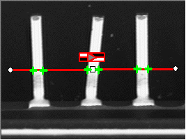
Point location. Contrast-based selection
The placement of a wedge gauge is defined by its nominal position (given by the coordinates of its center), its nominal inner and outer radius (inner and outer diameter), its breadth (difference between radii), the angular position from where it extents and its angular amplitude.
The Set member can distinguish between a full ring, a sector of a ring and a disk.
Each side of a wedge can have its own transition detection parameters and can be set to active or inactive with the ActiveEdges property. When a side is active, this means that:
- setting the value of a parameter only applies to the currently active sides;
- getting the value of a parameter yields a result only when the value of this parameter is the same for all active sides;
- only active sides are used for measurement and model fitting.
So different sides can have different parameters, and you can measure parallel arcs or oblique sides, or a corner point, instead of the whole wedge. The four sides are denoted by letters "a", "r", "AA" and "RR" respectively.
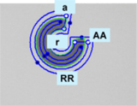
Naming conventions for the sides of a wedge gauge
Usage
Define and position the gauge, then use Measure to fit the lines.
To obtain the wedge properties, set the ActualShape property to TRUE to return the fitted line (instead of the nominal line position FALSE, default).
Alternatively,MeasuredWedge provides the results as an EWedge object.
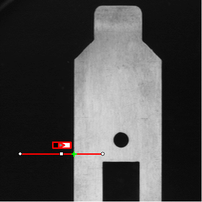
The placement of a line gauge is defined by its center coordinates, its length and its angle with respect to the X-axis. To constrain the line slope value, set Angle and KnownAngle.
Line fitting
Usage
Define and position the gauge, then use Measure to fit the lines. To obtain the line properties, set the ActualShape property to TRUEto return the fitted line (TRUE value) (instead of the nominal line position FALSE value, default).
Alternatively, MeasuredLine provides the results as an ELine object.
The placement of a circle gauge is defined by its nominal position (given by the coordinates of its center), its nominal diameter (or radius), the angular position from where it extents and its angular amplitude.
The Set member can distinguish between a full circle and an arc (the arc amplitude must be specified).
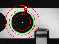
Circle fitting
Usage
Once the gauge has been defined and positioned, use Measure to trigger the circle fitting operation. To obtain the measurement results, set the ActualShape mode to TRUE. The ActualShape mode determines whether an inquiry returns the fitted circle (TRUE value) or the nominal circle position (FALSE value, default). The requested information is then retrieved by means of the circle properties.
Alternatively, MeasuredCircle provides the results as an ECircle object.
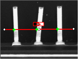
Finds the position of all transition points along a line segment probe that crosses one or several objects edges, and allows selecting the most relevant ones. Crosswise and lengthwise filtering can be activated for noise reduction.
Point location. Contrast-based selection
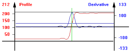
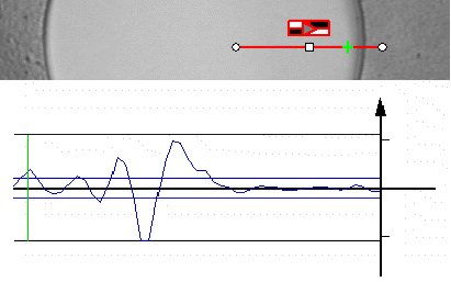
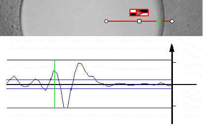
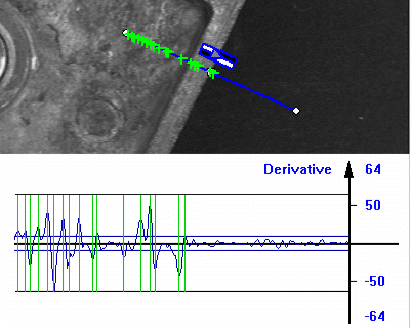
Point location principle (left) and S-shaped curve and its derivative (right)
On a linear profile extracted from an image, an edge appears as a transition from dark to light (or vice versa). When plotting pixel values along the gauge, this transition appears as an S-shaped curve. The first derivative of this curve exhibits a peak around the transition point. The better the contrast, the sharper the transition and the higher the peak.
EasyGauge extracts the pixel values along a profile (red curve) then uses peak analysis to determine the transition location. All the pixel values in the peak area are used to compute the transition location.
- Sub-pixel accuracy is only possible if the transition is surrounded by almost uniform regions of at least 2 pixels wide.
- BWB transitions have an increasing profile curve and the peak takes positive values. Otherwise, the curve decreases and the peak extends negatively.
- You cannot normally detect peaks using the default threshold value (20) as BWB or WBW transitions base the peak analysis on the gray level profile along the EPointGauge (or sample path) and not its first derivative.
EPointGauge contains all point measurement parameters, with default values that detect reasonably contrasted edges.
Center: Nominal point position (will normally be different before and after measurement).
Tolerance: Tolerance value and gauge orientations.
TransitionType, TransitionChoice, TransitionIndex: Peak selection strategies.
Threshold: Noise immunity.
MinAmplitude, MinArea: Peak strength.
Thickness, Smoothing: Local filter widths.
RectangularSamplingArea Sets sampling area (rectangular by default) to transverse filtering mode.
Measure: Measures the object.
- In single transition mode, Valid returns True when an appropriate point was found. To obtain measurement results, set ActualShape to True so that Center returns the located point. (False default value returns nominal point position ).
- In multiple transition mode, NumMeasuredPoints returns the number of points found,
GetMeasuredPoint returns an EPoint object which contains located point information.
An integer index between 0 and GetNumMeasuredPoints-1 must be passed.
GetMeasuredPeak: Returns EPeak containing the peak's Area and Amplitude, and the delimiting coordinates along the probe segment (Start, Length and Center values).
The threshold level is very important:
- Too high can cause significant peaks to be missed, and insufficient pixel values to achieve good precision.
- Too low can cause false peaks because of noise.
To resolve this dilemma, the EasyGauge peak selection mechanism can reject low contrast or false edges: transition strength is measured by peak amplitude and area. Every edge measurement determines peak amplitude and area. If either value falls below the minimum amplitude or minimum area, the peak is disregarded and no point is assumed at that location.
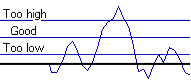
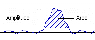
Threshold level selection (left) and Peak amplitude and area (right)
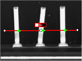
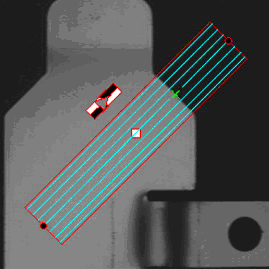
EasyGauge can measure several edge points in a single go and retrieve all results afterwards while in multiple transition mode.
Multiple transition (left) versus single transition (right)
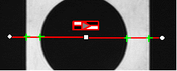
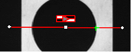
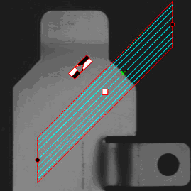
You can select the single most relevant transition based on 4 criteria: the highest peak, the peak with the largest area, the peak closest to the gauge center, or the N-th peak encountered starting from one tip of the gauge.

Best area (first image) and best amplitude choices (2nd image), closest (3rd image) and 3rd from the start (4th image)
Peak selection can also be refined by choosing the transition polarity: White to Black or Black to White (i.e. positive or negative peak), or indifferent.
Black to white, white to black or indifferent polarities
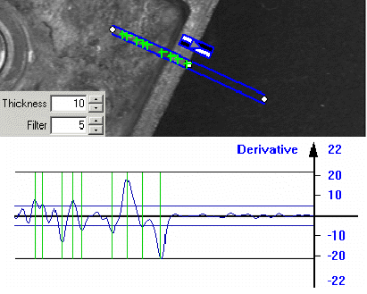
Pre-filtering the image locally can reduce noise effects.
Transverse (lengthwise) filtering averages several parallel lines when sampling the image.
Longitudinal (crosswise) uniform filtering can also be applied to the resulting profile curve.
Thick point gauge for filtering
Transverse filtering places parallel line segments in either a parallelogram or a rectangle (default). This behavior can be toggled.
Parallelogram mode is faster than rectangular if the angle is close to 0° or 90°, or thickness is less than 5. If thickness=1, no difference exists between the two modes.
thickness determines the number of parallel lines.
sampling area is the smallest region containing all the parallel line segments.
Rectangular sampling area (left) and Parallelogram sampling area (right)
The expected nominal position of a point gauge is specified by its center, orientation angle with respect to the X-axis, and length tolerancethat the point position can vary.
The results are the coordinates of the located points (the actual location) and the strength of the transition (amplitude and area).
Low values indicate a weak edge, possibly corresponding to an unreliable or inaccurate measurement.
The EasyGauge default parameters and working modes are good for clear edges. More complex situations may need parameter tuning.
| 1. Set the gauge point location and tolerance.
The center position and orientation are easy to decide based on a sample image or on coordinate considerations. The tolerance depends on the edge position variations. A larger tolerance increases the likelihood of hitting an edge, but it may be a false edge or extraneous feature. |
|
| 2. Decide whether noise reduction is required. Lay the gauge over the desired location and observe the profile curve and its derivative (play with the filtering parameters while looking at the plotted curve). The curve regularity gives an indication of the spread of the gray-level values. When these coefficients are set, the gray-level profile will not change anymore. |
|
| 3. Set the threshold value to be low enough for useful parts of the peaks to cover enough pixels (to achieve better sub-pixel accuracy), but not lower than the ambient image noise. | 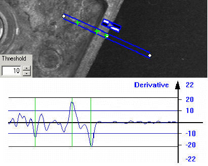
|
| 4. Remove weak or false edges using the list of peak amplitudes and areas. Plotting these values along with good and extraneous peaks can help find appropriate peak rejection limits. | 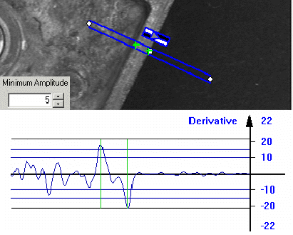
|
| 5. Choose whether all transition points are needed or just the most relevant. If all are required, they can be queried one after another. Otherwise, a point selection strategy should be chosen based on strength, order or transition polarity (black to white and/or conversely). | 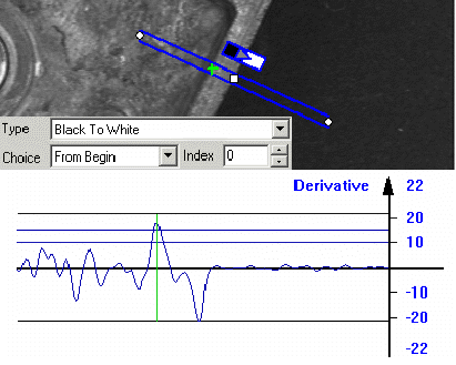
|
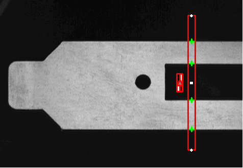
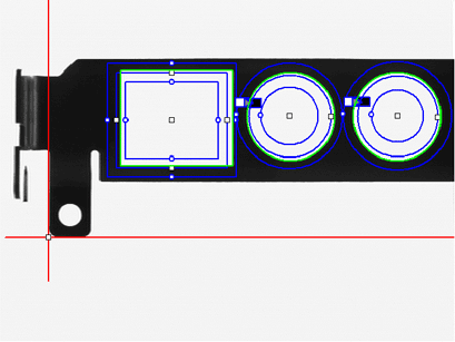
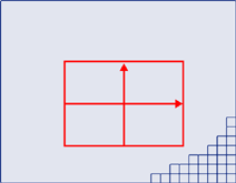
ELineGauge, ECircleGauge, ERectangleGauge, or EWedgeGauge predefined geometric models can be fit over the edges of an object. The targeted edge must be defined, and points sampled along it at regularly spaced point measurement gauges. Model fitting in the least square sense can be applied.
| Line: Measures position and orientation of straight edges. | 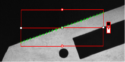 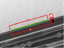
|
| Circle: Measures position and curvature of a circle or arc. | 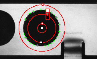 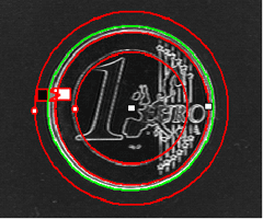 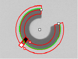
|
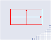
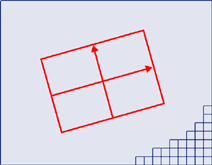
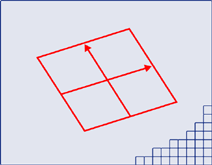
| Rectangle: Measures position, orientation and size of a rectangle. | 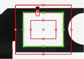 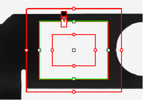
|
| Wedge: Measures position, orientation and size of a ring/ disk sector / curvilinear rectangle. | 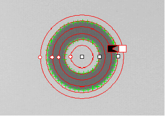 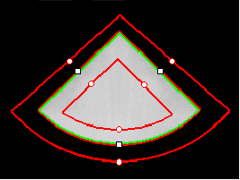 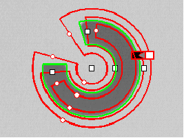
|
All gauge types share these common features:
| Point sampling | ||
|
Point gauges are placed along the edges and point measurement carried out at regularly spaced spots, which can be adjusted differently per side in rectangle and wedge gauges. All point measurement parameters and operating modes are available. SamplingStep sets the spacing of point location gauges along the model. NumSamples returns the number of points sampled during the model fitting operation. |
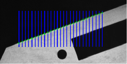
Sampling paths and sampled points |
|
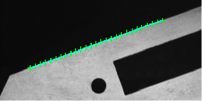
| Model fitting | ||
|
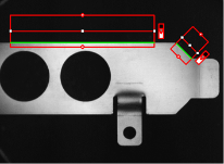
The model is adjusted to minimize error residue and provide the best edge parameter estimates. Rectangles and wedges have parallelism and concentricity constraints. Image shows sampled points and fitted line. |
|
|
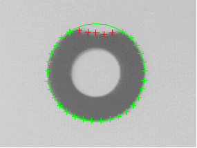
| Outlier rejection | ||
|
After model fitting, some points will be too far away from the fitted model and may harm location accuracy. EasyGauge can tag them as outliers to be ignored using the FilteringThreshold property. The outlier elimination process can be repeated several times using NumFilteringPasses. |
|
|
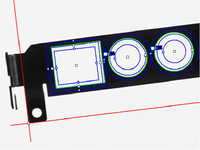
EasyGauge provides means to graphically interact with gauges to place and size them, combine them as a hierarchy of grouped items, and store/retrieve them and all working parameters to/from model files.
Draw gives a graphical representation of a gauge. Drawing is done with the current pen in the device context associated to the desired window. Depending on the operation, handles may be displayed.
An operator can drag a gauge interactively over an image. Several dragging handles are available.
- HitTest determines when the mouse cursor is over a handle. When it is, the cursor shape should be changed for feedback, and a drag can take place.
- Drag moves the handle and the corresponding gauge accordingly.
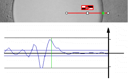
EasyGauge can Plot gray-level values along the sampled paths and/or its derivative - useful for parameter tuning.
Point measurement gauges can plot after calling Measure.
Model fitting gauges can plot after calling MeasureSample with an index argument that lies between 0 and GetNumSamples-1 (included).
To view the corresponding sampling path, use method Draw with mode EDrawingMode_SampledPath.
Measurement gauges can be grouped (their relative placement remains fixed) to form a dedicated tool that can be moved (translated and rotated) to follow the movement of inspected items / probes before computing measurements.
Attach associates a gauge to a mother gauge or EFrameShape object.
NumDaughters, GetDaughter, or Mother retrieves information relative to attached daughters or mother.
Detach, DetachDaughters dissociates the gauge or daughters from the mother.
| Field-of-view calibration | ||
|
Calibration establishes the relationship between real-world point coordinates and image pixels. A simple calibration model computes faster, a repeatable part position is easier to locate. |
|
|
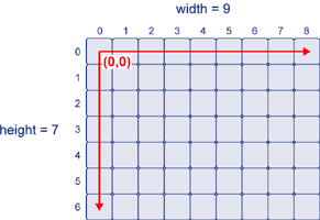
| The Raw sensor coordinate system starts from upper left and extends rightwards and downwards. The range of abscissae is 0 to width-1 and the range of ordinates is 0 to height-1 where integer coordinate values correspond to pixel centers. |
|
|
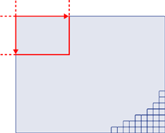
| The Centered sensor coordinate system starts at the center ([width-1]/2, [height-1]/2 in the Raw system) and extends rightwards and upwards. | 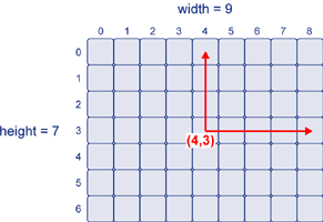
|
|
|
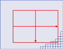
The real world 3D coordinates are defined in a 2D reference frame tied to a reference plane. The origin and direction of the axis are normally aligned with major features of the inspected parts. |
|
|
| Before World-to-Sensor Transform | ||
|
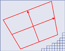
Before converting from world to sensor coordinates, sources of distortion should be eliminated:
|
||
| Effects of World-to-Sensor Transform | ||
|
|
|
|
|
|
|
|
|
|
|
|
|
|
|
|
|
|
|
|
|
|
|
|
|
|
|
The EWorldShape object can calibrate the whole field of view (in given imaging conditions with fixed camera placement and lens magnification), if the optical setup is modified.
EWorldShape computes appropriate calibration coefficients and transforms measurement gauges that are tied to it.
It can set world-to-sensor transform parameters, perform conversions from and to either coordinate system, determine unknown calibration parameters, and save the parameters of a given transform for later reuse.
After calibration EWorldShape can perform coordinate transform for arbitrary points using SensorToWorld and WorldToSensor to:
- measure non-square pixels and rotated coordinate axis.
- correct perspective and optical distortion, with no performance loss.
There are several ways to obtain the calibration coefficients:
To estimate the calibration coefficients either locate the limits of the field of view and divide the image resolution by the field of view size, or use the following procedure:
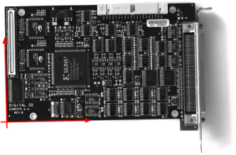
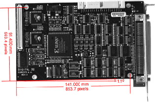
- Take a picture of the part to be inspected or a calibration target (e.g. rectangle).
- Locate feature points such as corners in the image (by the eye) and determine their coordinates in pixel units —let (i,j).
- Use the Euclidean distance formula to derive the calibration coefficient:
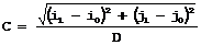
where C is a calibration coefficient, in pixels per unit, and D is the world distance between the corresponding points, in units. - For non-square pixels repeat this operation for pairs of horizontal and vertical points.
To estimate a skew angle, apply this formula to two points on the X-axis in the world system: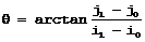
Estimating scale factors and skew angle
When the calibration coefficients are available, use SetSensor to adjust them and set the calibration mode, or set them individually using: SetSensorSize, SetFieldSize, SetResolution, SetCenter, SetAngle.
Locate at least 4 landmarks and obtain their coordinates in sensor (using image processing) and world coordinate systems (actual measurements). More landmarks give more accurate calibration.
The resulting pixels aspect ratio (X resolution/Y resolution) must be in the range [-4/3, -3/4] (or [3/4, 4/3]).
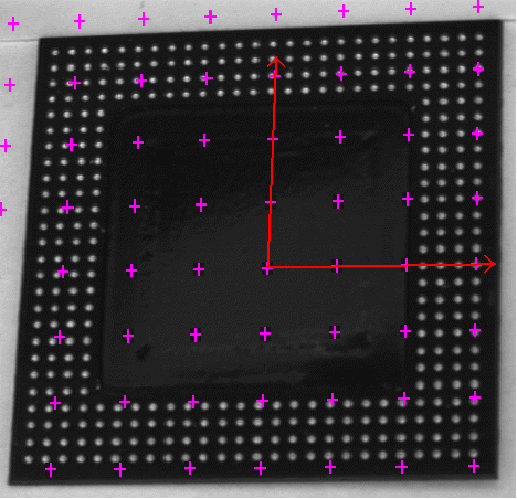
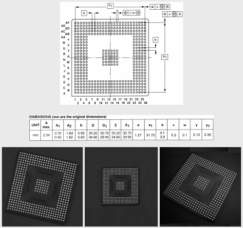
A calibration target can be automatically analyzed to get an appropriate set of landmarks. It is an easy way to achieve automatic calibration, provided an appropriate procedure is available to extract the desired landmark point coordinates.
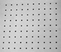
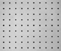
Open eVision relies on the use of a specific target holding a rectangular grid of symmetrical dots (of any shape)with no other object on the grid.
- Grab an image of the calibration target in such a way that it covers the whole field of view (or restrict the image of view to an ROI where only dots are visible).
- Apply blob analysis to extract the coordinates of the centers of the dots, as can be done by EasyObject.
- Pass all points detected to AddPoint (sensor coordinates only).
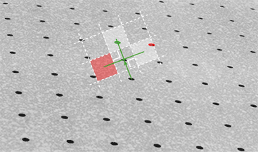
- Call RebuildGrid to reconstruct a grid to calibrate a field of view using an iterative algorithm which computes the world coordinates of each dot.
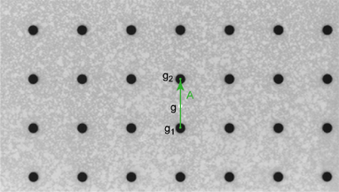
- The grid points nearest to the gravity center (g) of grid points are selected (g1 and g2) to form the first reference oriented segment, of length A.
- Starting from the extremity of the reference segment (g2), the algorithm determines 3 tolerance areas (white squares in the figure), in perpendicular directions. The tolerance areas are centered at a distance A (length of the reference segment) from (g2). They are square, with a side-length of A.
The algorithm searches for 1 neighboring point, in each of the 3 tolerance areas.
The grid will be correctly calibrated if each tolerance area contains a neighboring point. - The 3 perpendicular segments are the references of the next iterative searches. The algorithm goes back to step 2.
- Call Calibratethe landmark approach.
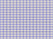
If the grid exhibits too much distortion, grid reconstruction does not work as expected. The following errors could happen:
- A tolerance area does not contain a neighboring point (red square in the figure).
- A tolerance area contains more than one neighboring point.
- The point in the tolerance area is not the correct one. For instance, the point might be diagonally connected (red point in the figure).
The field-of-view calibration model can be tuned using these parameters:
The sensor width and sensor height give the logical image size, in pixels (always integers).
The field-of-view (f-o-v) width and height give the actual image size, in length units, i.e. the size of the rectangle corresponding to the image edges in the world space. These values are related to the pixel resolution by the following equations:
f-o-v width = pixel width * sensor width
f-o-v height = pixel height * sensor height
or
sensor width = f-o-v width * horizontal resolution
sensor height = f-o-v height * vertical resolution
By default pixel height is not specified, the pixels are assumed to be square (pixel width = pixel height).
Anisotropic aspect ratio
The center abscissa (x) and ordinate (y) indicate the image origin point (world coordinates (0,0). Default is the image center.
The skew angle is the angle formed by the real-world reference frame (X-axis) and the image edge (horizontal). The default is no skew.
Skew angle
When the pixels are not square, the EWorldShape object can convert the angle between the world and sensor spaces.
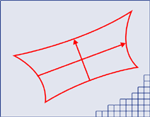
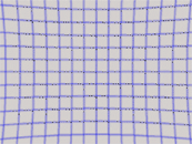
The perspective strength gives a relative measure of the perspective effect. The shorter the focal length, the larger the value.
Weak and strong perspective
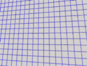
Distortion strength and GetDistortionStrength2 give a relative measure of radial distortion in the image corners, i.e. the ratio of image diagonal length with and without distortion.
Positive and negative distortion
Calibration mode, expressed as a combination of options, can be accessed via CalibrationModes.
Effect of the Calibration Coefficients
No calibration coefficient: All coefficients combined.
An EWorldShape object manages a field-of-view calibration context. Such an object is able to represent the relationship between world coordinates (physical units) and sensor coordinates (pixels), and account for the distortions inherent in the image formation process.
Image calibration is an important process in quantitative measurement applications. It establishes the relation between the location of points in an image (pixel indices) and the actual positions of those points in the real world, on the inspected item.
Calibration can be setup by providing explicit calibration parameters of the calibration model, or a set of known points (landmarks), or a calibration target.
The goal of calibration is twofold:
- To gain independence with respect to the viewing conditions (part placement in the field of view, lens magnification, sensor resolution, ...), letting you describe the inspected item once for all using absolute measurements.
Single model versus multiple viewing conditions
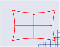
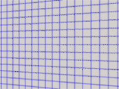
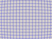
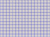
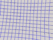
- To correct some distortion related to the imaging process (perspective effect, optical aberrations, ...).
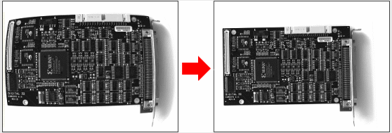
Removal of image distortion
The pixel indices in an image are usually integer numbers, but fractional values can occur when using sub-pixel methods. They are normally obtained by processing an image and locating known feature points. These values are called sensor coordinates.
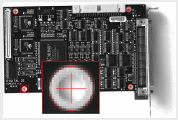
Feature point in sensor space
The world coordinates describe the location of points on the inspected item are expressed in an appropriate length measurement unit.
The world coordinates are actual dimensions, usually gathered from design drawings or by mechanical measurements.
They require a reference frame to be defined.
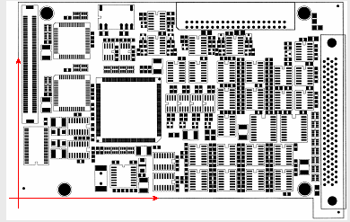
Reference frame in world space
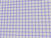
Unwarp an image using Unwarp, SetupUnwarp and UnwarpAfterSetup.
Using a lookup table before unwarping may speed up the process.
Distorted vs. Unwarped image